The Helmholtz equation#
In this tutorial, we will learn:
How to solve PDEs with complex-valued fields,
How to import and use high-order meshes from Gmsh,
How to use high order discretizations,
How to use UFL expressions.
Problem statement#
We will solve the Helmholtz equation subject to a first order absorbing boundary condition:
where \(k\) is a piecewise constant wavenumber, \(\mathrm{j}=\sqrt{-1}\), and \(g\) is the boundary source term computed as
for an incoming plane wave \(u_\text{inc}\).
import numpy as np
from mpi4py import MPI

import dolfinx
import ufl
This example is designed to be executed with complex-valued degrees of freedom. To be able to solve this problem, we use the complex build of PETSc.
import sys
from petsc4py import PETSc

if not np.issubdtype(PETSc.ScalarType, np.complexfloating):
    print("This tutorial requires complex number support")
    sys.exit(0)
else:
    print(f"Using {PETSc.ScalarType}.")
Using <class 'numpy.complex128'>.
Defining model parameters#
# wavenumber in free space (air)
k0 = 10 * np.pi

# Corresponding wavelength
lmbda = 2 * np.pi / k0

# Polynomial degree
degree = 6

# Mesh order
mesh_order = 2
Interfacing with GMSH#
We will use Gmsh to generate the computational domain (mesh) for this example. As long as Gmsh has been installed (including its Python API), DOLFINx supports direct input of Gmsh models (generated on one process). DOLFINx will then in turn distribute the mesh over all processes in the communicator passed to dolfinx.io.gmshio.model_to_mesh.
The function generate_mesh creates a Gmsh model on rank 0 of MPI.COMM_WORLD.
from dolfinx.io import gmshio
from mesh_generation import generate_mesh

# MPI communicator
comm = MPI.COMM_WORLD

file_name = "domain.msh"
generate_mesh(file_name, lmbda, order=mesh_order)
mesh, cell_tags, _ = gmshio.read_from_msh(file_name, comm,
                                          rank=0, gdim=2)
Info    : Reading 'domain.msh'...
Info    : 15 entities
Info    : 2985 nodes
Info    : 1444 elements
Info    : Done reading 'domain.msh'
Material parameters#
In this problem, the wave number in the different parts of the domain depends on cell markers, inputted through cell_tags.
We use the fact that a discontinuous Lagrange space of order 0 (cell-wise constants) has a one-to-one mapping with the cells local to the process.
W = dolfinx.fem.FunctionSpace(mesh, ("DG", 0))
k = dolfinx.fem.Function(W)
k.x.array[:] = k0
k.x.array[cell_tags.find(1)] = 3 * k0
import pyvista
import matplotlib.pyplot as plt
from dolfinx.plot import create_vtk_mesh
pyvista.start_xvfb()
pyvista.set_plot_theme("paraview")
sargs = dict(title_font_size=25, label_font_size=20, fmt="%.2e", color="black",
             position_x=0.1, position_y=0.8, width=0.8, height=0.1)

def export_function(grid, name, show_mesh=False, tessellate=False):
    grid.set_active_scalars(name)
    plotter = pyvista.Plotter(window_size=(700, 700))
    t_grid = grid.tessellate() if tessellate else grid
    renderer = plotter.add_mesh(t_grid, show_edges=False, scalar_bar_args=sargs)
    if show_mesh:
        V = dolfinx.fem.FunctionSpace(mesh, ("Lagrange", 1))
        grid_mesh = pyvista.UnstructuredGrid(*create_vtk_mesh(V))
        renderer = plotter.add_mesh(grid_mesh, style="wireframe", line_width=0.1, color="k")
        plotter.view_xy()
    plotter.view_xy()
    plotter.camera.zoom(1.3)
    plotter.export_html(f"./{name}.html", backend="pythreejs")
Show code cell source
grid = pyvista.UnstructuredGrid(*create_vtk_mesh(mesh))
grid.cell_data["wavenumber"] = k.x.array.real
export_function(grid, "wavenumber", show_mesh=True, tessellate=True)
2024-05-06 08:09:29.644 (   4.081s) [        823F1000]    vtkExtractEdges.cxx:435   INFO| Executing edge extractor: points are renumbered
2024-05-06 08:09:29.646 (   4.082s) [        823F1000]    vtkExtractEdges.cxx:551   INFO| Created 2214 edges
2024-05-06 08:09:29.666 (   4.103s) [        823F1000]    vtkExtractEdges.cxx:435   INFO| Executing edge extractor: points are renumbered
2024-05-06 08:09:29.667 (   4.104s) [        823F1000]    vtkExtractEdges.cxx:551   INFO| Created 2214 edges
Show code cell source
%%html
<iframe src='./wavenumber.html' height="700px" width="700px"></iframe>  <!--  # noqa, -->
Boundary source term#
where \(u_{inc} = e^{-jkx}\), the incoming wave, is a plane wave propagating in the \(x\) direction.
Next, we define the boundary source term by using ufl.SpatialCoordinate. When using this function, all quantities using this expression will be evaluated at quadrature points.
n = ufl.FacetNormal(mesh)
x = ufl.SpatialCoordinate(mesh)
uinc = ufl.exp(1j * k * x[0])
g = ufl.dot(ufl.grad(uinc), n) - 1j * k * uinc
Variational form#
Next, we define the variational problem using a 4th order Lagrange space. Note that as we are using complex valued functions, we have to use the appropriate inner product; see DOLFINx tutorial: Complex numbers for more information.
element = ufl.FiniteElement("Lagrange", mesh.ufl_cell(), degree)
V = dolfinx.fem.FunctionSpace(mesh, element)

u = ufl.TrialFunction(V)
v = ufl.TestFunction(V)
a = - ufl.inner(ufl.grad(u), ufl.grad(v)) * ufl.dx \
    + k**2 * ufl.inner(u, v) * ufl.dx \
    - 1j * k * ufl.inner(u, v) * ufl.ds
L = ufl.inner(g, v) * ufl.ds
Linear solver#
Next, we will solve the problem using a direct solver (LU).
opt = {"ksp_type": "preonly", "pc_type": "lu"}
problem = dolfinx.fem.petsc.LinearProblem(a, L, petsc_options=opt)
uh = problem.solve()
uh.name = "u"
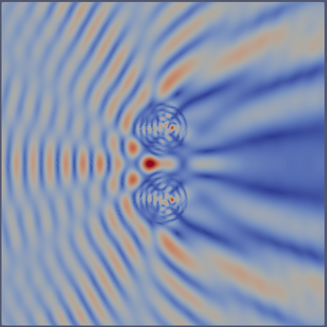
Postprocessing#
Visualising using PyVista#
topology, cells, geometry = create_vtk_mesh(V)
grid = pyvista.UnstructuredGrid(topology, cells, geometry)
grid.point_data["Abs(u)"] = np.abs(uh.x.array)
Show code cell source
%%html
<iframe src='./Abs(u).html' width="700px" height="700px">></iframe>  <!--  # noqa, -->
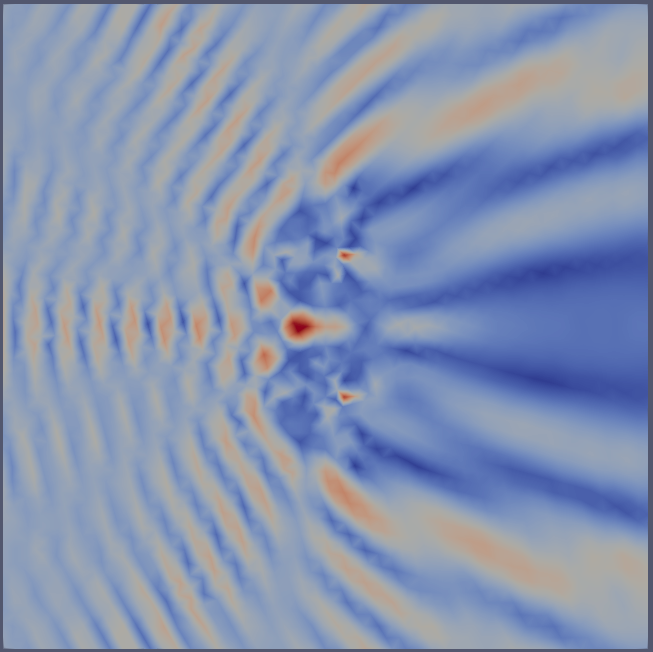
Post-processing with Paraview#
from dolfinx.io import XDMFFile, VTXWriter
u_abs = dolfinx.fem.Function(V, dtype=np.float64)
u_abs.x.array[:] = np.abs(uh.x.array)
XDMFFile#
# XDMF writes data to mesh nodes
with XDMFFile(comm, "out.xdmf", "w") as file:
    file.write_mesh(mesh)
    file.write_function(u_abs)
VTXWriter#
# VTX can write higher order functions
with VTXWriter(comm, "out_high_order.bp", [u_abs]) as f:
    f.write(0.0)